Hanoi PM$_{2.5}$ AI-Assisted Modeling Update (2018)
This page is intentionally separate from the 2026 forecasting experiments. It summarizes an AI-assisted reworking of an older Hanoi PM$_{2.5}$ dataset framed as a model-improvement exercise on the 2018 period rather than as the main 2026 operational forecasting study.
What This Entry Is
This graphic compares several model variants on the older Hanoi dataset and asks a narrower question:
- given a fixed historical PM$_{2.5}$ dataset
- how much can prediction error be reduced
- by moving from simple baselines to richer lag and feature-engineering setups
That makes it a modeling update on an older dataset, not the same thing as the later multi-horizon forecasting study built around operational-style forecast inputs.
Why It Is Separate
The 2026 forecasting page is about:
- explicit forecast horizons
- operationally framed weather inputs
- train/validation splits extending into 2025
- comparison against persistence for a deployment-style use case
This 2018 entry is about:
- model-improvement iteration on a historical dataset
- richer lag features and blending
- a tighter question of error reduction inside one data regime
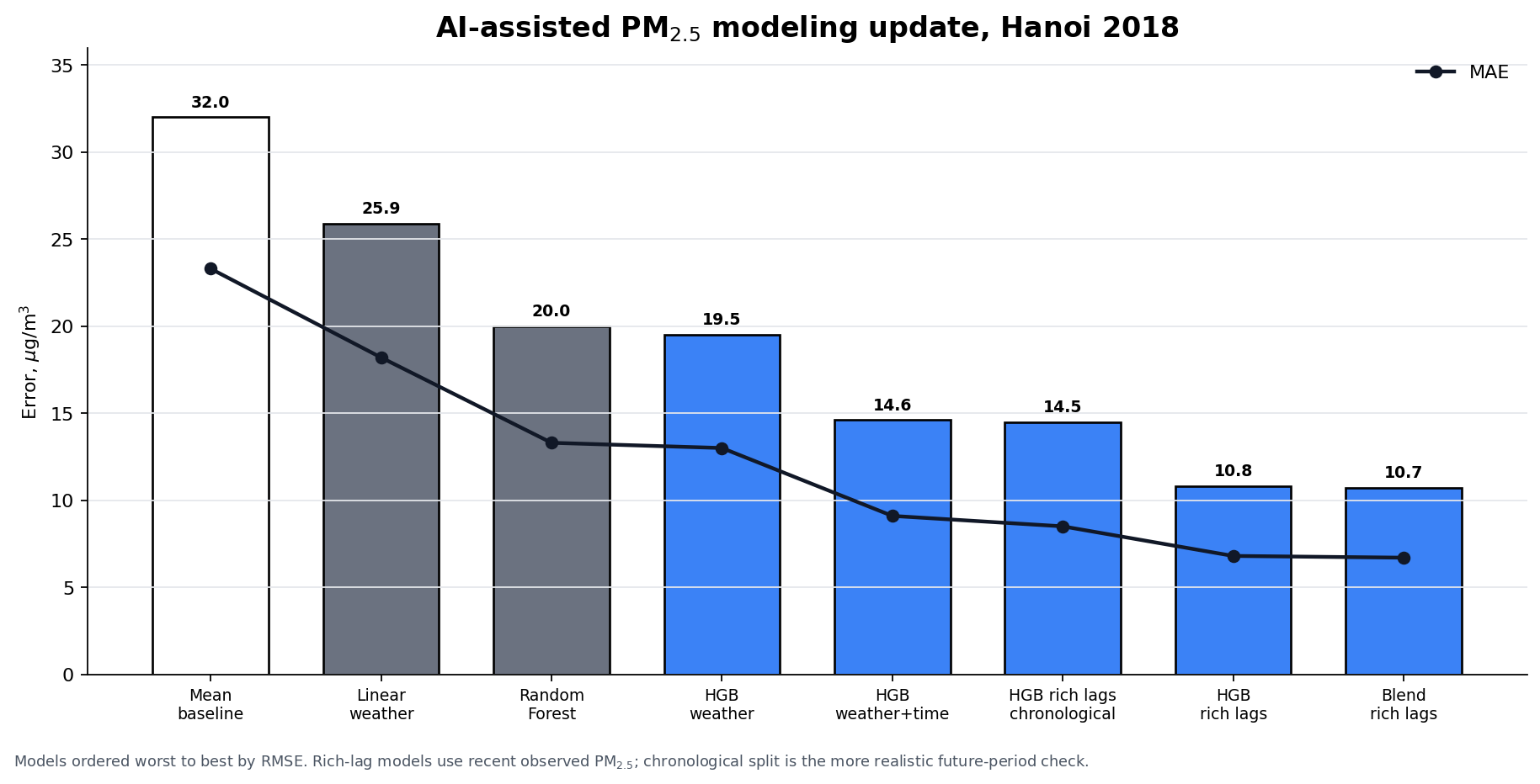
Reading the Figure
The strongest result in the chart is the Blend rich lags configuration, which pushes error down substantially relative to the mean baseline and simple weather-only models.
The broad progression shown in the figure is:
- mean baseline performs worst
- adding weather helps
- richer non-linear models help more
- lag-heavy and blended models improve further
- chronological testing remains the more realistic check
Model Metrics in the Figure
The plotted figure comes from the later 3.3 rework notebook, which reports all three headline metrics on a common random split, plus one chronological hold-out check.
Table ordered from worst to best RMSE (showing the progression of model improvements):
| Label in figure | Split | RMSE ($\mu g/m^3$) | MAE ($\mu g/m^3$) | R$^2$ |
|---|---|---|---|---|
| Mean baseline | random | 32.0 | 23.3 | -0.001 |
| Linear weather | random | 25.9 | 18.2 | 0.345 |
| Random Forest | random | 20.0 | 13.3 | 0.610 |
| HGB weather | random | 19.5 | 13.0 | 0.629 |
| HGB weather+time | random | 14.6 | 9.1 | 0.793 |
| HGB rich lags chronological | chronological | 14.5 | 8.5 | 0.814 |
| HGB rich lags | random | 10.8 | 6.8 | 0.883 |
| Blend rich lags | random | 10.7 | 6.7 | 0.886 |
Key observations:
Blend rich lagsachieves the lowest error (10.7 $\mu g/m^3$), representing a 66.6% improvement over the mean baseline.Random Forest(20.0 $\mu g/m^3$) performs slightly worse thanHGB weather(19.5 $\mu g/m^3$) but significantly better than linear weather models.- The progression from simple baselines → weather-only → time features → rich lags shows clear, systematic improvement.
HGB rich lags chronological(14.5 $\mu g/m^3$) provides the more realistic forward-in-time evaluation, showing higher error than random-split validation but still a 54.7% improvement over baseline.
Random Forest in Context
The original 2018 regression notebook included a standalone RandomForestRegressor trained on the same mixed meteorology dataset. Rerunning this model with the same train/test split (33% test, random_state=2020) gives complete metrics:
| Model | RMSE ($\mu g/m^3$) | MAE ($\mu g/m^3$) | R$^2$ | Position |
|---|---|---|---|---|
| Random Forest | 20.0 | 13.3 | 0.610 | 3rd of 8 models |
This places Random Forest:
- 22.8% better than
Linear weather(RMSE 25.9) - Slightly behind
HGB weather(RMSE 19.5), but similar performance tier - 46.5% worse than the best model,
Blend rich lags(RMSE 10.7) - R$^2$ of 0.610 indicates it explains 61% of PM$_{2.5}$ variance using weather alone
The key insight is that Random Forest provides a solid non-linear baseline, but the major gains come from:
- Adding temporal structure (HGB weather+time: RMSE 14.6, R$^2$ 0.793)
- Incorporating lag features that encode recent PM$_{2.5}$ state (HGB rich lags: RMSE 10.8, R$^2$ 0.883)
- Ensemble blending across multiple strong learners (Blend rich lags: RMSE 10.7, R$^2$ 0.886)
What Each X-Axis Label Means
The chart is easiest to read if each label is treated as a different modeling scope rather than just a different algorithm.
Mean baseline
- Predicts the overall mean PM$_{2.5}$ concentration.
- Uses no meteorology, no time structure, and no recent PM$_{2.5}$ history.
- Purpose: anchor the chart with a trivial no-skill baseline.
Linear weather
- Model: linear regression.
- Inputs: meteorological variables only from the mixed 2018 dataset
comb_PM25_wind_Hanoi_2018_v3.csv. - Data scope: the underlying notebook describes this as a mixed meteorology set rather than a live forecast product.
- Purpose: show what a simple linear weather-only relationship can do.
HGB weather
- Model:
HistGradientBoostingRegressor. - Inputs: the same weather-only feature scope as
Linear weather. - Purpose: test whether a stronger non-linear learner helps even before adding time or lagged PM$_{2.5}$ information.
HGB weather+time
- Model:
HistGradientBoostingRegressor. - Inputs: weather variables plus calendar structure such as hour-of-day, day-of-week, day-of-year, and month encodings.
- Purpose: test whether descriptive temporal patterning improves a weather-only model.
HGB rich lags
- Model:
HistGradientBoostingRegressor. - Inputs: weather, time structure, and recent observed PM$_{2.5}$ lag features and rolling summaries.
- Purpose: move from pure weather regression toward short-horizon forecasting / nowcasting.
Blend rich lags
- Model: weighted blend of
HistGradientBoosting,Random Forest, andExtra Trees. - Inputs: the same rich-lag feature set as
HGB rich lags. - Purpose: see whether a small ensemble can reduce error slightly beyond a single strong learner.
HGB rich lags chronological
- Model:
HistGradientBoostingRegressor. - Inputs: the same rich-lag feature scope.
- Evaluation difference: trained on the earlier part of 2018 and tested on the later part of 2018.
- Purpose: show the more realistic forward-in-time result, rather than a notebook-style random holdout.
Why the Best Bar Sits in the Middle
The x-axis is not ordered from worst to best.
It is ordered as a modeling story:
- trivial baseline
- simple weather-only model
- stronger weather-only model
- weather plus temporal structure
- rich-lag forecasting models
- stricter chronological check at the end
So Blend rich lags appears near the middle-right because the figure is organized by feature scope and evaluation regime, not by ranking. The final bar is reserved for the more realistic chronological test, which is conceptually the last step in the comparison.
Recovered Result Summary
The closest surviving writeup frames this modeling pass as a test of a simple question: do strong descriptive temporal patterns in Hanoi PM$_{2.5}$ translate into useful predictive power by themselves?
The recovered answer is no.
Later notes describe the temporal signal in the underlying Hanoi series as strong in descriptive terms:
- seasonal variability was the dominant pattern, with
32%coefficient of variation - diurnal variability was present but weaker, about
8.4% - weekday effects were negligible, about
1.1%
That descriptive structure looked promising, but the predictive tests collapsed when the model relied mostly on temporal structure rather than recent PM$_{2.5}$ state and weather drivers.
Main Quantitative Takeaway
The recovered benchmark table from the later paper notes is:
| Model family | Features | RMSE ($\mu g/m^3$) | R$^2$ | Readout |
|---|---|---|---|---|
| Temporal-only (basic) | 8 | 34.2 | -0.25 | failed badly |
| Temporal-only (enhanced) | 19 | 34.0 | -0.23 | failed badly |
| Persistence | 1 | 14.7 | n/a | strong naive baseline |
| Full baseline | 76 | 12.7 | 0.82 | best recovered reference |
That is the core modeling lesson behind this figure:
- temporal-only models were about
2.3xworse than persistence - they were about
2.7xworse than the fuller baseline - adding recent PM$_{2.5}$ history and weather physics mattered far more than seasonal averages or clock-time patterns
Why the Better Models Improved
The recovered notes consistently point to the same explanation:
- temporal features mostly encode climatology
- richer lag features encode current pollution state
- weather features encode dispersion and trapping conditions
- blended models perform better because they combine both recent state and physical drivers
In plain terms, a temporal-only model can say “December evenings are usually polluted”, but it cannot tell whether a specific evening is clean after rain or extreme during a stagnant inversion. The stronger models improve because they are closer to the actual state of the atmosphere.
Interpretation for the 2018 Entry
This is why the page should be read as a model-improvement note, not just a chart gallery item. The figure documents an early but useful conclusion:
- descriptive patterns are real
- descriptive patterns alone are not enough for forecasting
- richer lag engineering and weather-aware models are where the meaningful gains came from