PM$_{2.5}$ Sensor Collocation Campaign Draft
This page is a draft reconstruction for local review in Jekyll. The overall campaign structure is now much clearer, but some file-to-sensor assignments are still being verified.
This page reconstructs an archived long-running field campaign in Hanoi, Vietnam. The original dynamic-correlate framing is no longer appropriate because the live service is gone. What still matters is the study design: an mlab co-location unit operating several low-cost PM sensors, with nearby anchor devices such as Dylos DC1100 Pro, Dylos DC1700, and IQAir AirVisual Node Pro, plus an attempt to tie the field comparisons back to earlier BAM-referenced calibration work.
Working campaign model
Based on the recovered CSV exports and archived notes, the campaign now appears to have had three layers:
- A dedicated
mlabco-location unit that housed the main low-cost PM sensor setup. - Several larger nearby monitors sitting outside but close to that unit, including
Dylos DC1100 Pro,Dylos DC1700, andIQAir AirVisual Pro/Node. - Additional device-specific logging streams and side experiments that were related to the broader measurement effort but not always part of the same physical enclosure.
That distinction matters. One CSV file in the recovered database is often best interpreted as a sensor/setup/script stream, not simply a single instrument.
What this campaign was trying to do
Most low-cost PM$_{2.5}$ writeups appear months after the field work ends. That lag weakens the connection between the measurement campaign and what readers can actually inspect. The original dynamic-correlate post tried to shorten that gap by publishing rolling comparison plots while the experiment was still active.
That framing is no longer appropriate because the live charts are gone. The more durable story is this:
- A set of low-cost optical PM sensors were run side by side in ambient Hanoi air within the
mlabco-location unit. - A Dylos DC1100 Pro was used as a more established mid-tier anchor device for day-to-day comparison.
- The campaign also leaned on a separate earlier study that compared PMS7003 and SDS011 against a MetOne BAM-1020 reference station.
- The practical question was not whether a cheap sensor could become a BAM, but whether a cheap sensor could track real variation consistently enough to be useful after local adjustment.
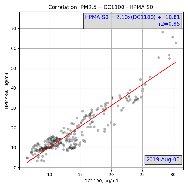
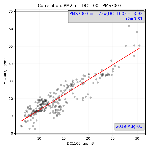
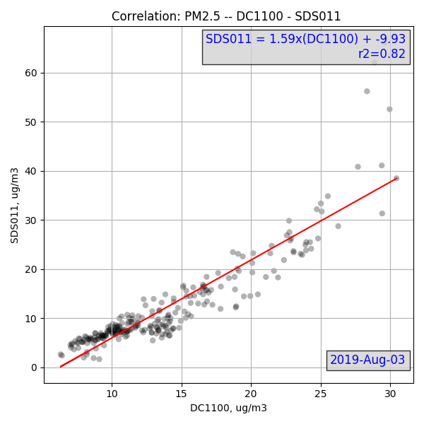
The preserved figures from this phase focus on three direct pairings:
- Dylos DC1100 Pro vs Honeywell HPMA115S0
- Dylos DC1100 Pro vs Plantower PMS7003
- Dylos DC1100 Pro vs Nova Fitness SDS011
The broader campaign notes also mention adjacent observations with Dylos DC1700 and IQAir AirVisual Node Pro, but the archived static figures that survive for this post are centered on the DC1100 Pro.
Recovered data streams
The current reconstruction groups the recovered CSV exports as follows.
Core co-location unit
mlab_p1.csvmlab_p2.csvmlab_p3.csvmlab_pms5003.csv
These appear to be the strongest candidates for the main co-location box / platform logs.
Nearby anchor devices
dylos.csvdc1700.csvairvisual.csv
These are interpreted as larger nearby monitors that sat outside but close to the co-location unit.
Device-specific streams related to the broader campaign
honeywell.csvhpma_01.csv,hpma_02.csv,hpma_03.csvsds011_08db.csv,sds011_75ee.csv,sds011_a307.csv,sds011_a30b.csv,sds011_a327.csvzh03b_001.csv,zh03b_01.csv,zh03b_02.csv,zh03b_03.csv
These are likely sensor-specific logs produced by the same broader measurement effort, but not necessarily all inside the same enclosure at the same time.
Separate experiments or context streams
mask_exp.csv,mask_one.csv— mask filtration experimenthepa_filter.csv— indoor HEPA experimentmh_z19.csv,mh_z19_two.csv— CO$_2$ monitoringsolcast_actual.csv,solcast_forecast.csv— solar/energy contextdust_work.csv— unresolved and needs additional inspection
This classification is provisional, but it is already strong enough to prevent the co-location post from mixing unrelated experiments into the main narrative.
Recovered Data Summary
Instead of a raw file manifest, the recovered data is grouped by operational role to support future analysis:
1. Core Co-Location Unit (Jan 2019 – May 2022)
The primary low-cost sensor platform operated continuously, capturing long-term PM trends.
- Data streams:
mlab_p1,mlab_p2,mlab_p3,mlab_pms5003 - Coverage: Over 3 years of active monitoring.
2. Mid-Tier Anchors (May 2019 – Aug 2022)
Three more stable commercial monitors provided a baseline for comparison.
- Devices: Dylos DC1100 Pro, Dylos DC1700, IQAir AirVisual Node Pro.
3. Sensor-Specific Cohorts (Mar 2020 – May 2021)
A dense deployment block testing multiple sensors of the same model simultaneously.
- Devices: Honeywell HPMA115S0, Nova SDS011, Winsen ZH03B.
- Purpose: Assess intra-model variance and reliability.
4. Separate Contextual Studies
Additional logs captured alongside the main campaign, requiring independent analysis:
- Mask & Filtration:
mask_exp,mask_one,hepa_filter - Indoor Environment:
mh_z19(CO$_2$ monitoring) - Energy/Solar Context:
solcast_actual,solcast_forecast
Note: The legacy file dust_work.csv contains invalid early timestamps and requires preprocessing before use. An empty export mlab_onboard.csv was also recovered but contains no data.
Mid-Tier Sensor Time Coverage and Correlation
As a first reconstruction target, I aligned the three surviving mid-tier monitors:
Dylos DC1100 Profromdylos.csvDylos DC1700fromdc1700.csvIQAir AirVisualfromairvisual.csv
Shared coverage
Using 15-minute bins, the common three-way overlap window is:
2019-08-25 11:30:00to2022-07-31 03:00:0089,055aligned bins

Exploratory correlation approach
The three devices do not expose identical fields, so this first-pass comparison uses a pragmatic alignment:
- DC1100: fitted PM$_{2.5}$-like field already present in
dylos.csvaspm2_5_f - DC1700: exploratory PM$_{2.5}$ proxy using the same simple Dylos-family heuristic,
(small - large) / 100 AirVisual: directpm25field from the device export
This is good enough for a first behavioral comparison, but it should still be treated as exploratory, especially on the DC1700 side where we are deriving a proxy rather than reading a native PM$_{2.5}$ field.
Pairwise correlation
| Pair | Pearson r |
|---|---|
DC1100 fit vs DC1700 proxy | 0.9313 |
| DC1100 fit vs AirVisual PM$_{2.5}$ | 0.8457 |
| DC1700 proxy vs AirVisual PM$_{2.5}$ | 0.8897 |

The immediate takeaway is that the three mid-tier devices appear to move together strongly over the shared long-term window, even before any deeper calibration or event-level filtering.
Hour-of-Day Stability
I treated hour-of-day stability as a diagnostic check. For each hour 00:00 through 23:00, I pooled the full campaign and recomputed the three pairwise correlations.
The result is reassuring: no hour-of-day bucket fell below r = 0.2 for any pair. In other words, there is no evidence here for a permanently bad nightly or daytime operating window that should be dropped wholesale.

What the deeper diagnostics show
The global correlation hides several important behaviors that are more useful than the single r values alone.
1. No meaningful lag at 15-minute resolution
Scanning lags from -120 to +120 minutes showed that all three pairs peak at 0-minute lag. In other words, at the campaign time scale used here, none of the three mid-tier devices appears to be consistently delayed relative to the others.

2. Agreement is not equally stable month to month
Monthly correlation is mostly strong, but not uniform. A few examples stand out:
2019-08starts very strong:DC1100vsAirVisualreaches0.93682021-04is also very strong, withDC1100vsAirVisualat0.92572021-09weakens noticeably:DC1100vsAirVisualdrops to0.67862022-06and2022-07degrade sharply forDC1100against the others, suggesting a late-period drift, setup change, or data-quality issue rather than a stable three-device relationship2022-02should not be overread because only20aligned bins survived that month

3. Agreement is stronger in dirty-air periods than in cleaner air
Splitting the aligned data by AirVisual PM$_{2.5}$ tertiles shows a clear pattern:
- Low regime
0.0to23.0:DC1100vsAirVisualis0.5294 - Mid regime
23.5to51.0:DC1100vsAirVisualis0.4610 - High regime
51.05to564.2:DC1100vsAirVisualrises to0.6722
The same pattern holds for DC1700 and AirVisual, where agreement improves from 0.5245 in the low regime to 0.7910 in the high regime. That is typical of PM sensors: they often agree more clearly when pollution events dominate the signal and less clearly near cleaner-background conditions.
4. DC1100 and DC1700 are the tightest pair
Across the full aligned dataset, the strongest relationship remains DC1100 versus DC1700 at 0.9313, and that relationship stays high across most months and concentration regimes. That supports the idea that the two Dylos-family devices are behaving as a coherent pair, even if one still needs a better PM conversion model.
What to do with this
For the three mid-tier devices, the next truly useful products are not more global scatter plots. They are:
- a late-period quality check focused on
2022-05to2022-07 - an event-based comparison using high-PM episodes only
- a better DC1700 conversion than the simple
(small - large) / 100proxy
That would move the analysis from “these sensors correlate” to “when and why they agree or diverge.”
Available overlap windows
The archived watermarked plots were probably cumulative correlation views up to the stamped date, not the full extent of the surviving dataset. The recovered CSV archive suggests that a much broader correlation range should be possible.
Long overlap windows already visible in metadata
mlab_p1.csv,mlab_p3.csv, andmlab_pms5003.csvoverlap withdylos.csvfrom 2019-05-28 to 2022-05-25.- Those same
mlab_*streams overlap withdc1700.csvfrom 2019-08-10 to 2022-05-25. - They overlap with
airvisual.csvfrom 2019-08-25 to 2022-05-25. - A dense multi-sensor block exists from 2020-03-17 to 2021-05-20, where
mlab_*, multipleSDS011streams, multipleZH03Bstreams, and nearby anchor devices are all present.
That means the August 2019 archived figures are probably only one visible slice of a larger campaign rather than the natural limit of the data.
Why this matters
For reconstruction, it is reasonable to treat the surviving images as campaign snapshots, while the CSV archive should make it possible to build:
- longer correlation windows for
mlabversusdylos - longer correlation windows for
mlabversusdc1700 - longer correlation windows for
mlabversusairvisual - multi-sensor overlap studies during the March 2020 to May 2021 deployment block
Likely parallel streams, not simple duplicates
Some file groups have names that differ only by a few hexadecimal-like digits, especially the SDS011 and ZH03B files. At first glance they could be mistaken for duplicate exports. The recovered timing and value patterns suggest something else: they are more likely parallel devices of the same sensor family.
SDS011 observations
sds011_a327.csv,sds011_a30b.csv, andsds011_a307.csvall begin on 2020-03-01, but not at the exact same time.sds011_08db.csvandsds011_75ee.csvbegin on 2020-03-17, again only a few seconds apart.- The
a3xxfiles have roughly 63-64 second cadence in the sampled rows. - The
08dband75eefiles have roughly 143-145 second cadence in the sampled rows. - When paired within tight time windows, the readings are similar but not identical, which argues against them being duplicate dumps of one sensor stream.
In other words, the differing suffixes are best read as device identifiers or logger-specific stream names, not just accidental copies.
ZH03B observations
zh03b_01.csv,zh03b_02.csv, andzh03b_03.csvrun in nearly the same overall window.zh03b_02.csvandzh03b_03.csvoften start within seconds of each other and can match on some rows, but they also diverge often enough to look like separate sensors exposed to the same air rather than the same file saved twice.
This is useful because it supports a richer reconstruction: the archive may preserve not just one representative low-cost PM sensor per family, but several same-model devices running in parallel.
Devices involved
| Tier | Device | Role in the campaign |
|---|---|---|
| Low-cost | Plantower PMS7003 | Optical PM sensor with PM1 / PM$_{2.5}$ / PM$_{10}$ output and size bins |
| Low-cost | Nova Fitness SDS011 | Optical PM sensor with PM$_{2.5}$ / PM$_{10}$ output; some deployments appear to have used a custom Python driver |
| Low-cost | Honeywell HPMA115S0 | Optical PM sensor with industrial-style documentation |
| Mid-tier | Dylos DC1100 Pro | Particle counter used as a practical comparison anchor |
| Mid-tier / adjacent | Dylos DC1700 | Nearby comparison monitor in the broader campaign |
| Consumer finished device / adjacent | IQAir AirVisual Node Pro | Nearby comparison monitor in the broader campaign |
| Reference | MetOne BAM-1020 | Earlier FEM-grade station used for calibration attempts |
Why use Dylos as an anchor?
The Dylos DC1100 Pro sits in an interesting middle ground. It is much more expensive than hobby sensors like PMS7003 or SDS011, but still far below laboratory-grade reference instruments. It also reports particle counts rather than a directly standardized PM$_{2.5}$ mass concentration, so part of the campaign was devoted to exploring how those counts might be converted into PM$_{2.5}$-like values.
That makes Dylos useful for two separate reasons:
- It is a stable, self-contained field device that can run for long periods and capture variation in particle counts.
- It provides a bridge between cheap raw optical sensors and the more formal BAM-based calibration work.
The same logic likely applied to DC1700 and AirVisual in the broader campaign: they were not BAM instruments, but they provided more operationally complete reference points than bare UART PM modules alone.
SDS011 software note
The campaign also appears to have relied on customized software around some of the low-cost sensors. A useful lead is the bi2air/SDS011 Python project, described as a Python interface for the Nova Fitness SDS011 sensor with support for running multiple sensors at once. That is consistent with a campaign architecture where several SDS011 devices were logged in parallel rather than as a single one-off bench setup.
Converting Dylos counts to PM$_{2.5}$
The archived campaign preserved five approaches for converting Dylos small-particle counts into PM$_{2.5}$ estimates. The author ultimately chose the GRIMM-based fit for the rolling charting, but the page documented the alternatives explicitly.
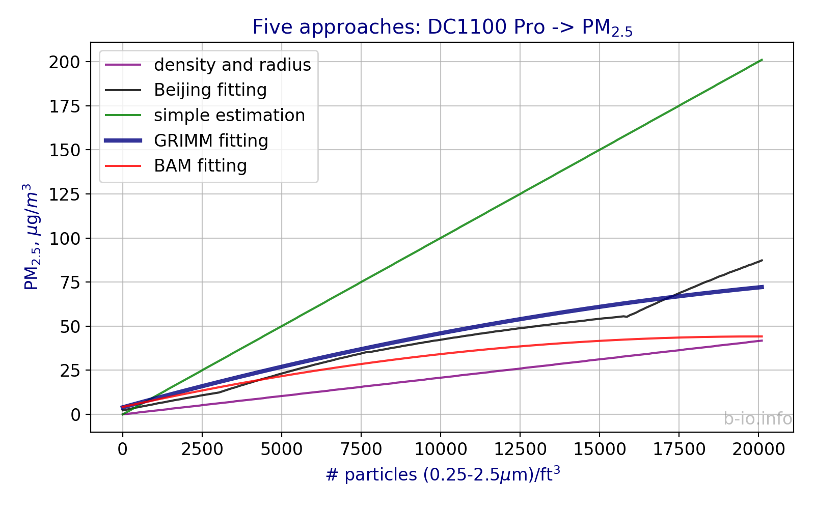 Five preserved conversion approaches for Dylos DC1100 Pro particle counts. The original live page used the GRIMM-based fit for charting.
1. Particle density and representative size assumption
Assume particle density:
\[\rho = 1.65 \times 10^{12}\ \mu g/m^3\]Assume representative particle radius:
\[r = 0.44\ \mu m\]Mass of one particle:
\[m = \rho \times \frac{4}{3}\pi r^3\]which gives approximately:
\[m \approx 5.89 \times 10^{-7}\ \mu g\]Dylos reports small and large counts per 0.01 ft^3, so the fine-particle count estimate is:
and the implied PM$_{2.5}$ mass estimate becomes:
\[PM_{2.5} = (\text{small} - \text{large}) \times 2.08 \times 10^{-3}\ \mu g/m^3\]This is physically interpretable but rests on strong assumptions about density and representative size.
2. Beijing AQI fit
The archived notes also preserved a polynomial fit associated with the Beijing Dylos-to-AQI workflow:
\[AQI_{US} = 3.31\times10^{-22}x^5 - 1.04\times10^{-16}x^4 + 1.19\times10^{-11}x^3 - 5.85\times10^{-7}x^2 + 0.016x + 9.43\]This approach maps raw Dylos counts to AQI first, then back-calculates PM$_{2.5}$ from AQI breakpoints.
3. Simple estimation
A simpler field heuristic used in the original post was:
\[PM_{2.5} = \frac{\text{small} - \text{large}}{100}\]The archived notes explicitly say this was hard to verify independently.
4. GRIMM EDM-180 fit
The AQ-SPEC / GRIMM-based fitting used in the original charting was:
\[PM_{2.5} = -8\times10^{-12}x^2 + 5\times10^{-5}x + 3.98\]with archived goodness-of-fit:
\[R^2 = 0.815\]5. MetOne BAM-1020 fit
The BAM-based fit preserved in the notes was:
\[PM_{2.5} = -1\times10^{-11}x^2 + 4\times10^{-5}x + 4.17\]with archived goodness-of-fit:
\[R^2 = 0.632\]This matters because it ties the Dylos-centered campaign back to the earlier BAM comparison work, even though the Dylos itself was not a reference instrument.
Static correlation snapshots from the campaign
The original page was meant to update continuously. What survives are static monthly snapshots from the August 2019 run.
Raw pairwise count relationships
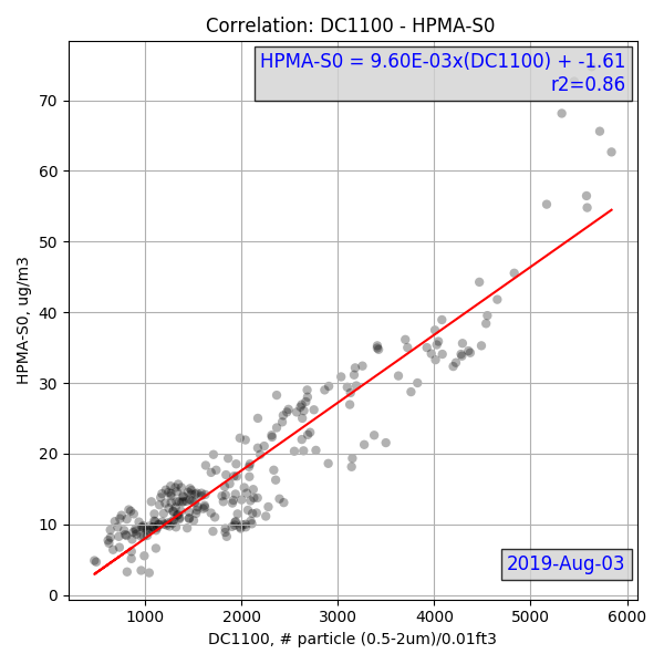
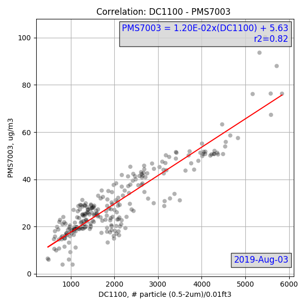
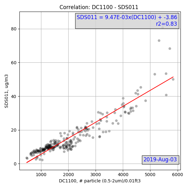
PM$_{2.5}$-adjusted pairwise comparisons
In the original post, the -ad plots indicated PM$_{2.5}$ values adjusted using coefficients from the BAM-linked calibration work.
What this campaign adds beyond the BAM page
The earlier Low-Cost PM$_{2.5}$ Sensors page is the better place for the strict reference-station calibration story. That page compares PMS7003 and SDS011 directly with the US Embassy Hanoi MetOne BAM-1020 over about 60 days.
This campaign adds a different layer:
- More sensors operating together in the same broader field effort
- A dedicated co-location unit rather than only one-off sensor checks
- A mid-tier field device used as an operational anchor
- A practical attempt to answer whether the cheap sensors move with the same air, even when absolute PM$_{2.5}$ remains uncertain
- A preserved example of how one might build rolling co-location comparisons before formal publication
In other words, the BAM page answers: How far are these sensors from a reference?
This page answers: When multiple optical sensors are placed into the same field campaign, do they move together well enough to support interpretation?
Limits of the archived material
- The original page used a live iframe/dashboard that no longer exists, so this reconstruction is necessarily static.
- The current write-up combines archived posts, CSV export metadata, and memory-based campaign reconstruction, so some sensor pinning still needs verification.
- The preserved figures emphasize DC1100-centered pairwise comparisons, not a full synchronized matrix including DC1700 and IQAir.
- The Dylos-to-PM$_{2.5}$ conversion methods are attempts and fits, not universal physical truth.
- The BAM comparison for Dylos was indirect in this reconstructed page; the strictest BAM work is still better represented in the earlier calibration study.
- At least one recovered file,
dust_work.csv, contains obviously bad early timestamps and should not be treated as clean campaign data without further filtering.
Takeaways
- This was a real long-running field campaign, not just a one-day gadget comparison.
- The campaign was valuable because it combined a dedicated co-location unit, nearby anchor devices, and an attempt to stay connected to a reference-station calibration.
- The original “dynamic” framing is historical; the durable value now is the co-location design and the preserved static correlation figures.
- The strongest next step is to verify the remaining file-to-sensor mappings and rebuild the campaign as a reproducible data article rather than a live dashboard.
Related pages
- Low-Cost PM$_{2.5}$ Sensors — BAM-based calibration of PMS7003 and SDS011
- AQI Calculation Guide — AQI breakpoints and PM$_{2.5}$ conversion context
References
- AQ-SPEC / South Coast AQMD field evaluation for Dylos DC1100 Pro
- MetOne BAM-1020 reference station material
fijnstofmeter.comDylos validation notes- myhealthbeijing Dylos AQI conversion spreadsheet
bi2air/SDS011Python interface for Nova Fitness SDS011 sensors- Original archived
dynamic-correlateanddust-sensornotes from b-io.info
Draft reconstructed from archived 2019-2022 material. Live charting removed; campaign structure and preserved static figures retained.