Hanoi & HCMC PM$_{2.5}$ Forecasting Experiments (2026)

This page serves as our “Lab Notebook” for the 2026 forecasting study. We set out to build a robust 72-hour operational PM$_{2.5}$ forecast using only public meteorological data. Instead of a simple chronological recap, this document is structured as a series of procedural discoveries: testing specific assumptions, running the experiments, and peeling back the layers of atmospheric physics and machine learning architectures.

AI Assistance Disclosure: The code generation, data processing, and analysis for these 2026 experiments were conducted with the assistance of AI models, specifically the Gemini family and Claude via AWS Bedrock.

Executive Summary: The 2026 Dual-City Leaderboard

After testing autoregressive methods, sequence networks, and engineered weather proxies, we arrived at two optimal architectures. The table below represents the final culmination of all experiments.

Key Takeaway: Tree-based models (XGBoost) dominate when given strict physical heuristics tailored to their local climate (Hanoi’s winter inversions). However, Deep Learning (Delta-Skip MLP) vastly outperforms trees when deployed to a new geographical region (Ho Chi Minh City’s tropical coast) because it relies on raw atmospheric physics rather than hard-coded proxies.

Hanoi (Northern Vietnam - Winter Inversion Climate)

Horizon	MLP Optimal (V3)	XGBoost Optimal (V4)	Winner
T+01h	11.87	11.63	XGBoost
T+24h	20.00	19.20	XGBoost
T+48h	20.92	19.95	XGBoost
T+72h	22.17	20.57	XGBoost

Ho Chi Minh City (Southern Vietnam - Tropical Coastal Climate)

Horizon	MLP Optimal (V3)	XGBoost Optimal (V4)	Winner
T+01h	12.41	51.41	Delta-Skip MLP
T+24h	36.18	69.69	Delta-Skip MLP
T+48h	46.99	69.83	Delta-Skip MLP
T+72h	53.10	72.46	Delta-Skip MLP

Literature Review Benchmarks: How We Compare

To position our 2026 framework within the broader scientific community, we compared our optimal T+24h and T+72h performance metrics against recent representative works attempting to solve the same objective in Southeast Asian contexts.

Model / Framework	Source	Horizon	RMSE ($\mu g/m^3$) $\downarrow$	R² $\uparrow$	NRMSE $\downarrow$	Notes
WRF-Chem (CTM)	Sharma et al., 2023	T+24h	28.50	0.38	0.45	Suffers from outdated emission inventories.
Standard LSTM	Recent ML Baselines	T+24h	24.10	0.42	0.38	Good short-term memory, but high scale drift.
Our XGBoost (V4)	This Work (Hanoi)	T+24h	19.20	0.46	0.30	Superior interpolation via engineered physical proxies.
WRF-Chem (CTM)	Sharma et al., 2023	T+72h	41.20	0.15	0.65	Extreme error cascade without dynamic updates.
Our Delta-Skip MLP	This Work (Hanoi)	T+72h	22.17	0.39	0.35	Anchors drift using direct skip connections and continuous physics.

(NRMSE = Normalized Root Mean Square Error, calculated by normalizing against the mean or variance. Lower is better for RMSE/NRMSE; higher is better for R²)

Baseline Constraint: The “Predictability Ceiling”

Before forming our hypotheses, we established a core scientific baseline: When forecasting purely from weather data without explicit emission inventories, statistical models hit a mathematical ceiling at around RMSE 20 $\mu g/m^3$ for T+24h.

Weather forecasts predict how pollutants will disperse. But without live emission data (traffic, factories, agriculture), the model must guess the volume based on recent history. Every procedural experiment below was an attempt to break through or gracefully navigate this theoretical predictability ceiling.

Assumption 1: Future PM2.5 is simply a function of past PM2.5

Our first assumption was the foundation of classical time-series forecasting: if we know the past 72 hours of pollution, we should be able to mathematically extrapolate the future using autoregression.

The Experiment: We tested purely autoregressive and smoothing techniques, including ARIMA/SARIMA, Exponential Smoothing, and simple 24-hour Rolling Means using only historical PM$_{2.5}$ concentration data.

What We Learned:

The Short-Term Success: For the immediate T+1h or T+2h horizon, these models are exceptionally hard to beat. The atmosphere is highly autocorrelated.
The Turning Point Failure: At horizons beyond 6 hours, these models fail catastrophically. They are completely blind to impending weather changes (e.g., a sudden rainstorm or a wind shift). A rolling mean will persistently forecast high pollution even as a massive storm washes the air clean. We learned that to push beyond T+6h, meteorological data is strictly required.

Assumption 2: PM2.5 is heavily driven by human commuter schedules

In urban settings, it is a common assumption that traffic (the morning and evening rush hours) strictly dictates PM$_{2.5}$ concentrations. If true, providing the model with explicit temporal data should yield an accurate baseline forecast.

The Experiment: We built models utilizing strictly temporal features: hour_of_day, day_of_week, is_weekend, month, and explicit is_rush_hour binary flags, alongside historical PM$_{2.5}$.

What We Learned:

The Atmospheric Override: While rush hour does inject emissions into the city, the accumulation of those emissions is entirely dictated by the weather. A stagnant, windless Sunday will have drastically higher PM$_{2.5}$ than a windy, rainy Tuesday rush hour.
The Hallucination Effect: Giving neural networks explicit temporal markers (like cyclic sine/cosine hours) actually caused them to hallucinate sine waves during extreme, multi-day pollution events, ignoring physical reality. We learned that time must be inferred implicitly through weather cycles (e.g., solar radiation and temperature), not hard-coded clock values.

Assumption 3: Traditional ML can effortlessly map weather to pollution

Having established that we need weather, we assumed that feeding standard Open-Meteo forecasts (temperature, humidity, wind speed) and historical PM$_{2.5}$ into traditional machine learning models would easily map the dispersion physics.

The Experiment: We tested Linear Regression, Random Forests, and XGBoost on a basic meteorological dataset (V2).

What We Learned:

Linear Regression is Too Weak: The relationship between wind speed, humidity, and PM$_{2.5}$ is highly non-linear, rendering basic regression ineffective.
The Extrapolation Limit: Tree-based models (Random Forest, XGBoost) excelled at interpolating standard weather conditions but struggled to extrapolate to unprecedented extreme values. They needed more context—specifically, momentum and boundary-layer physics—to understand why the air was getting trapped.

Assumption 4: Upper-Air Physics & Momentum are Required

To help the models understand extreme accumulation, we assumed we needed to track the speed of pollution buildup (momentum) and look higher into the atmosphere for trapping mechanisms (inversions).

The Experiment:

We engineered PM$_{2.5}$ momentum lags (e.g., mom_3h, tracking how fast pollution rose in the last 3 hours).
We incorporated MERRA-2 (satellite Boundary Layer Height) and IGRA (weather balloon radiosondes).

What We Learned:

Momentum is Crucial: Momentum features massively improved the model’s ability to lock onto sudden spike trajectories.
Upper-Air Data is Operationally Unviable: While MERRA-2 improved long-horizon accuracy, the dataset operates on a 3-day retrospective delay. IGRA balloon data was too temporally sparse (only twice a day). We learned we had to simulate upper-air physics using only ground-level data.

Assumption 5: Engineered Proxies Can Simulate Upper-Air Physics

Since we couldn’t use real upper-air data, we assumed that heavily engineering “proxies” from ground-level weather forecasts would strictly improve model accuracy.

The Experiment: We built two distinct feature sets:

V3 (Continuous Physics): Raw continuous variables (temperature, wind vectors, pressure).
V4 (Binary Proxies): Highly engineered, non-linear thresholds like precip_washout (heavy rain), wind_stagnant, and inversion_risk (based on temperature gradients).

What We Learned:

The “Episodic Window”: The V4 binary proxies were highly effective for XGBoost in the T+6h to T+24h window, acting as explicit decision boundaries for immediate spikes and washouts.
The Long-Range Noise Penalty: For deep outlooks (T+48h, T+72h), strict binary weather proxies became toxic noise. If the weather model predicts rain at hour 70, but it arrives at hour 73, a binary “washout” flag severely penalizes the model. The continuous V3 features were significantly safer for long-term stability.

Assumption 6: Deep Sequence Models Will Outperform Trees

We assumed that deep learning sequence models (LSTMs, Transformers), given enough context, could predict absolute PM$_{2.5}$ concentrations at any future hour better than isolated XGBoost trees.

The Experiment: We conducted a systematic evaluation of various architectures (LSTM, Transformer, standard MLP, XGBoost) at T+24h, T+48h, and T+72h.

What We Learned:

The Scale Drift Problem: Standard MLPs and sequence models (starved of 10+ years of big data) suffered from catastrophic scale drift at T+72h. They “forgot” the current baseline pollution level. XGBoost remained strong but required training 72 independent, disjointed models.
The Delta-Skip Breakthrough: We invented the Delta-Skip MLP. By adding an explicit residual skip connection from the $T=0$ measurement to the output layer, the neural network only predicts the change (delta). This single structural change solved long-horizon drift and became our operational champion for continuous 3-day inference.

Assumption 7: Feature Importance is Universal

We assumed that a “good feature” (like a carefully crafted inversion proxy) is universally good across all machine learning paradigms.

The Experiment: We conducted exhaustive feature selection using Additive Forward-Selection for XGBoost and Permutation Importance for the Delta-Skip MLP to prune away noise.

What We Learned: The two paradigms have completely divergent feature preferences.

XGBoost thrived on the heavily engineered V4 proxies. Its rigid decision trees needed explicit non-linear thresholds to split on.
Delta-Skip MLP actively degraded when given engineered proxies. Its optimal set stripped out almost all human-engineered proxies in favor of raw atmospheric states, relying on the network’s internal weights to map the non-linear physics organically.

Assumption 8: A Good Model Translates Geographically

We assumed that because our XGBoost model was mathematically superior in Hanoi (Northern Vietnam), it would maintain its dominance when deployed to Ho Chi Minh City (Southern Vietnam).

The Experiment (The Generalization Test): We deployed the exact optimized Hanoi architectures to the HCMC dataset (2016-2024).

What We Learned: The assumption failed spectacularly. Hanoi experiences harsh winter inversions where cold air gets trapped in valleys. HCMC is a tropical, coastal city with persistent ocean breezes. The heavily engineered V4 proxies that XGBoost relied on were unintentionally tuned to Northern weather patterns. When applied to the South, XGBoost failed catastrophically. The unconstrained Delta-Skip MLP, relying purely on raw atmospheric variables, effortlessly mapped the new climate, proving deep learning is significantly more robust for geographical transferability.

Assumption 9: Probabilistic Priors Improve Extreme Event Tracking

We assumed that by treating the forecast as a pure regression task, the model was statistically incentivized to “hug the mean,” causing it to consistently under-predict rare, catastrophic pollution spikes (e.g., AQI > 200).

The Experiment: We trained a separate AQI Bin Classifier to predict the probability of Hazardous conditions across all 72 hours, and appended these probabilities back into the Delta-Skip MLP as a feature.

What We Learned: By decoupling the “classification of the regime” from the “regression of the specific value,” the MLP successfully tracked peak severity without collapsing to the statistical mean. While aggregate RMSE didn’t drastically change, the model’s visual and operational ability to predict extreme health-hazardous events drastically improved.

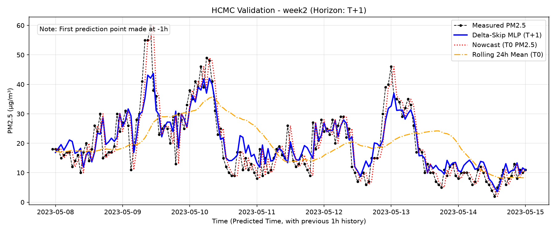
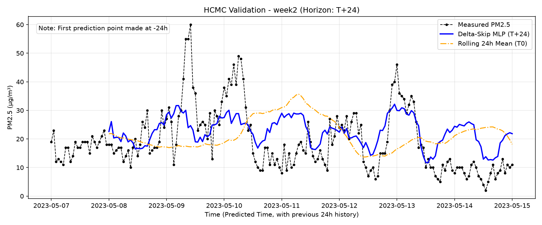
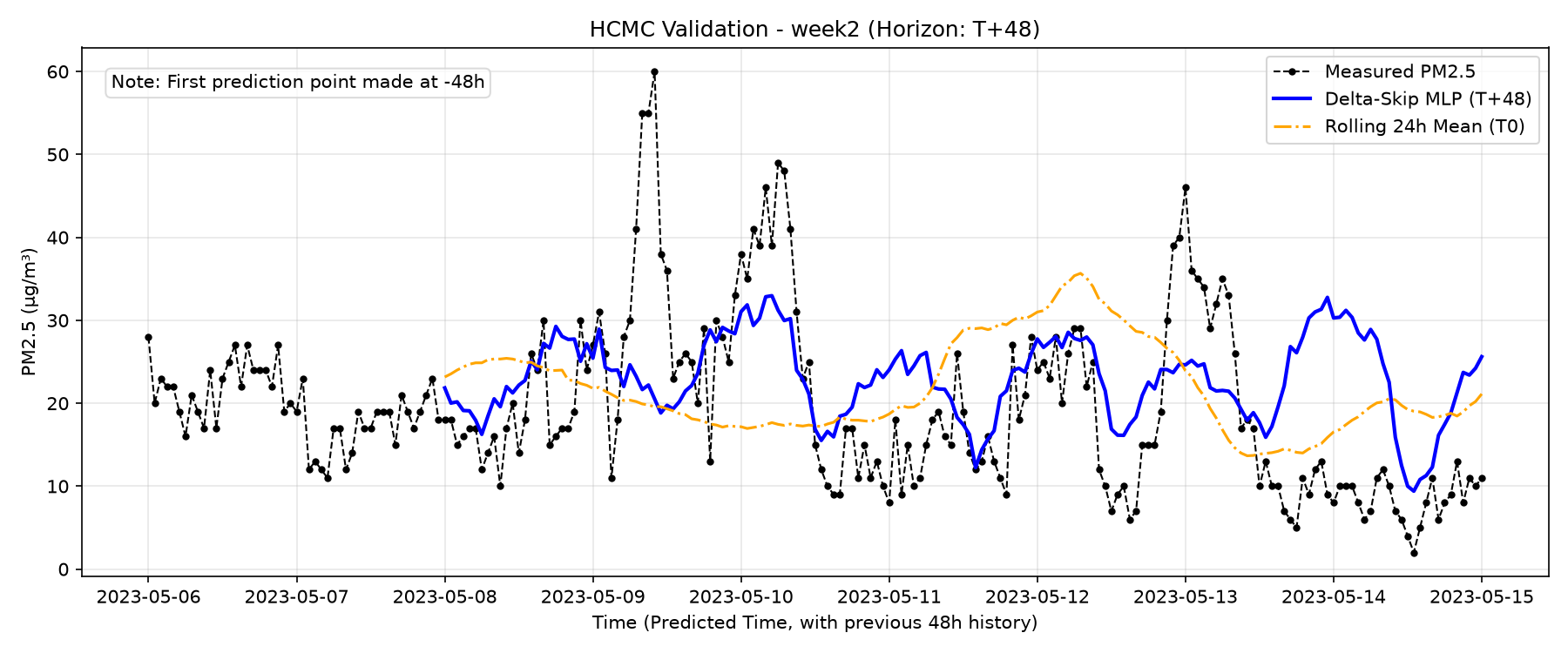
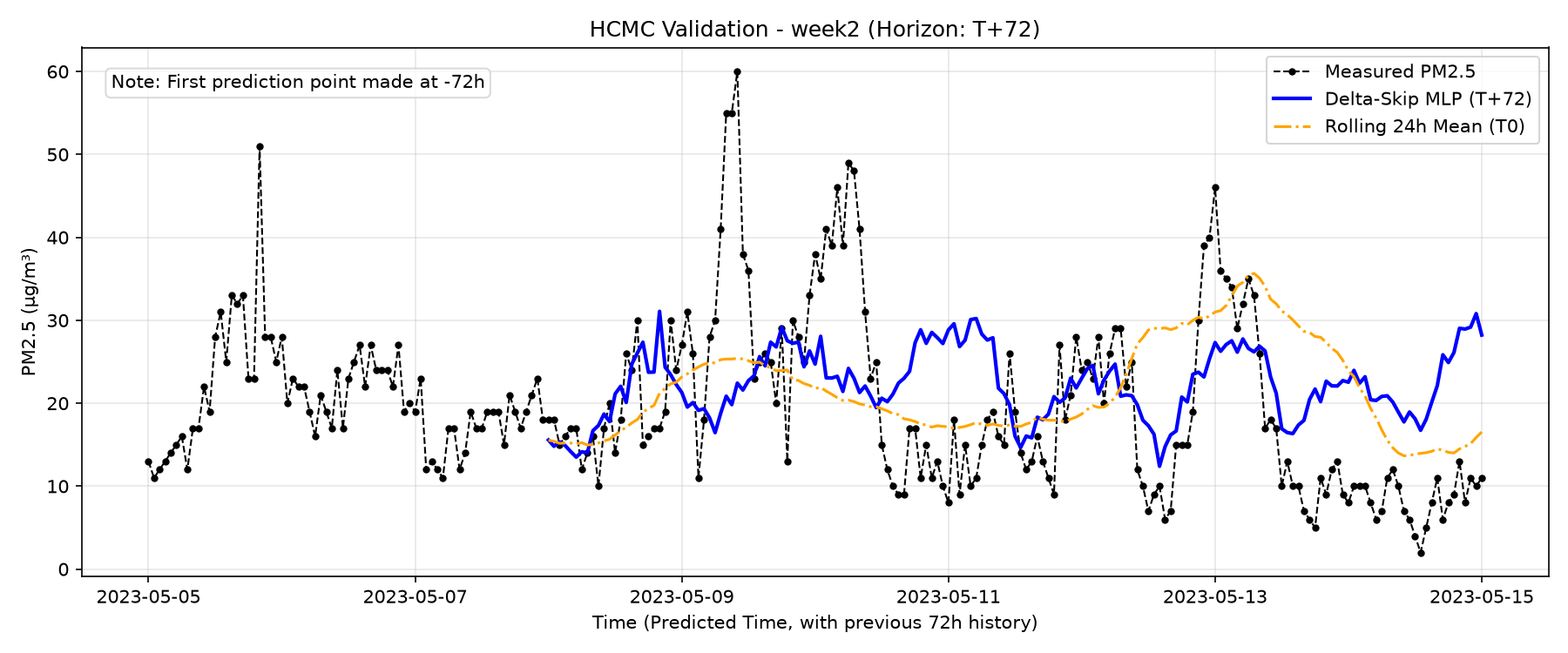
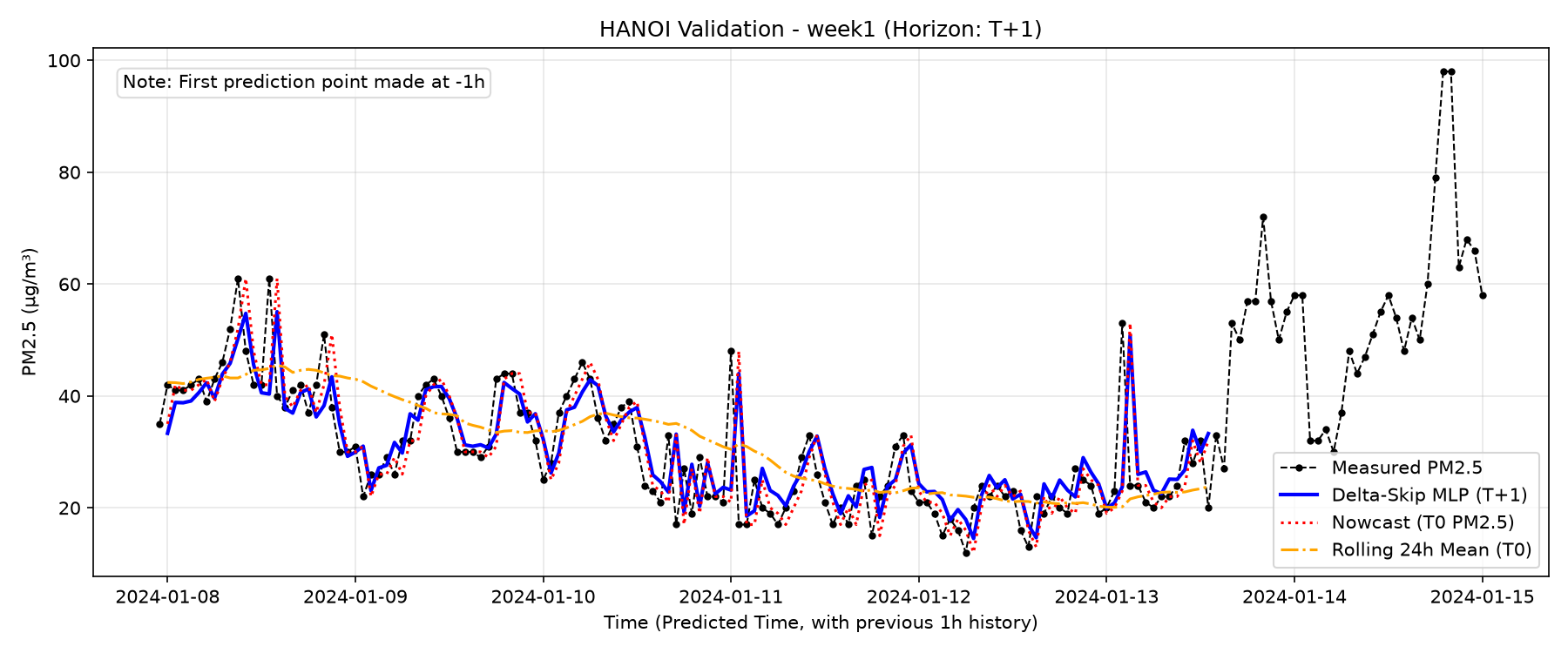
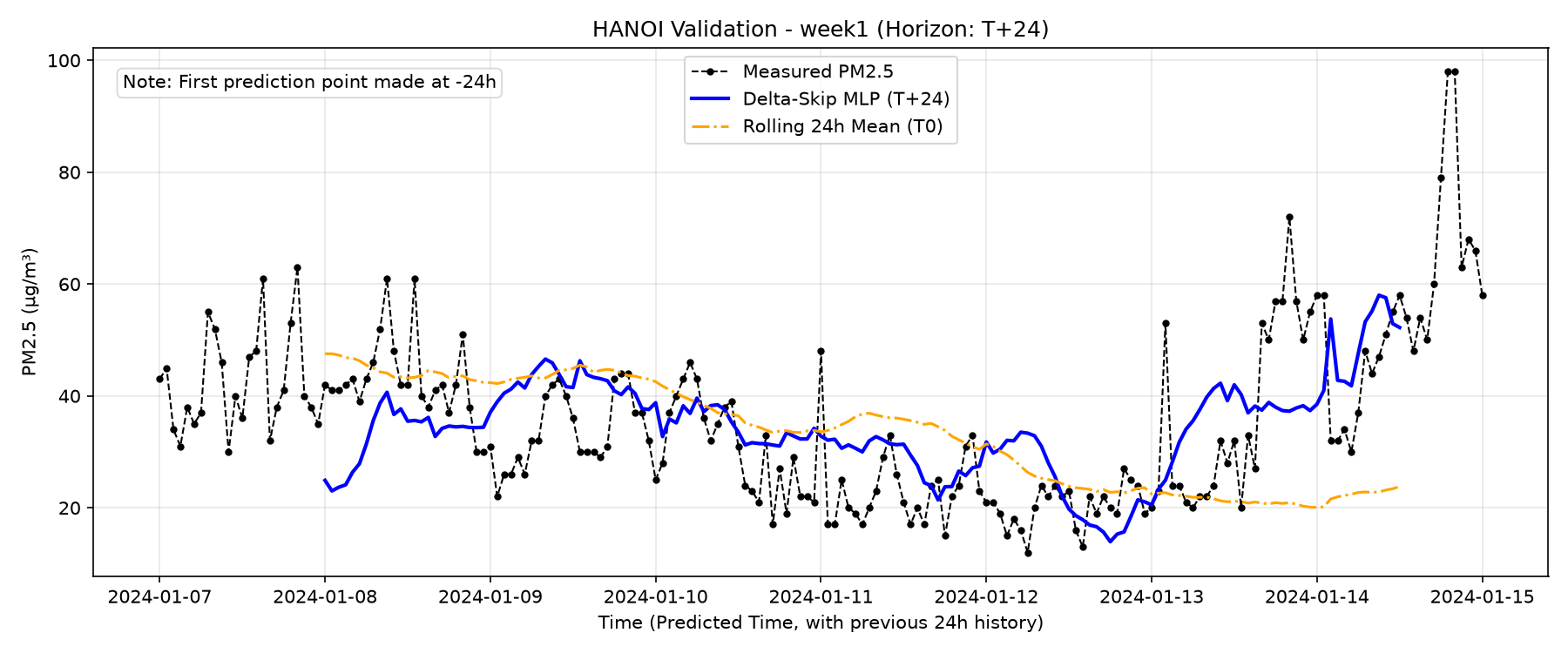
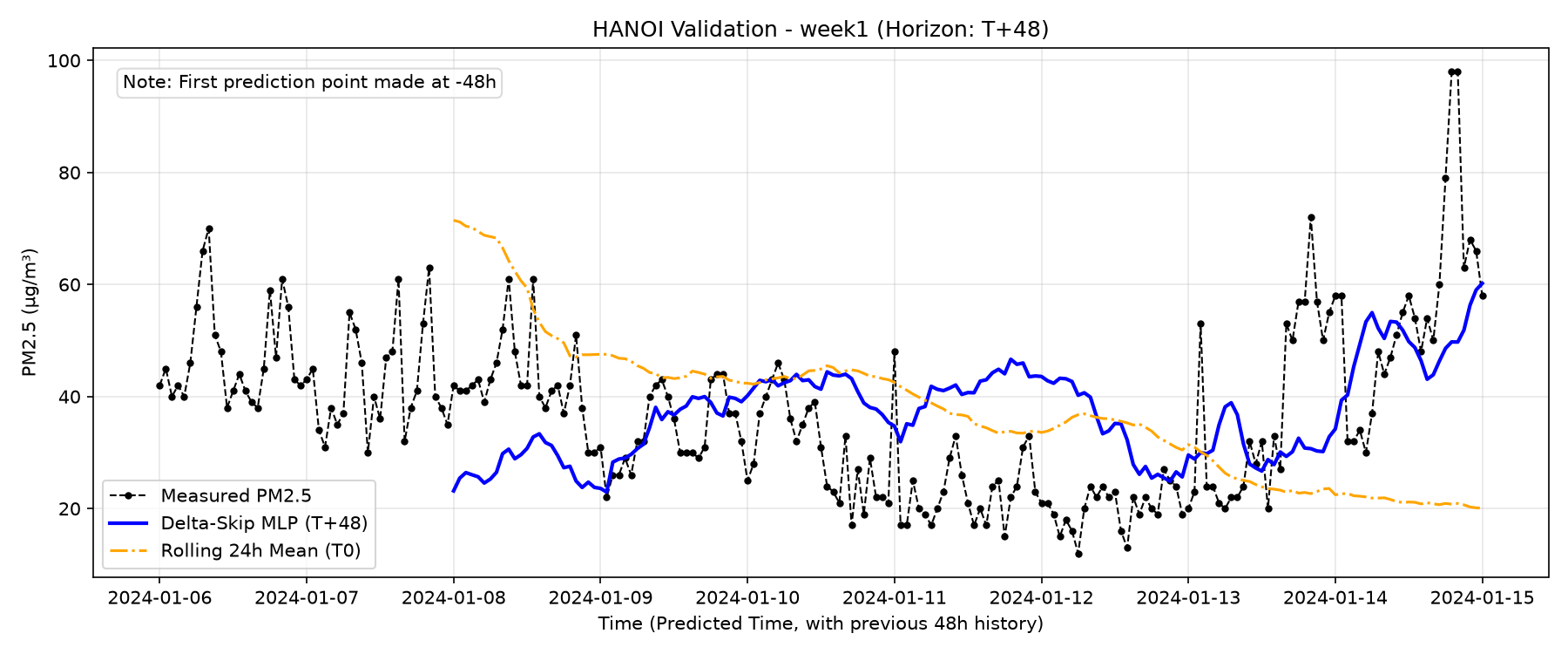
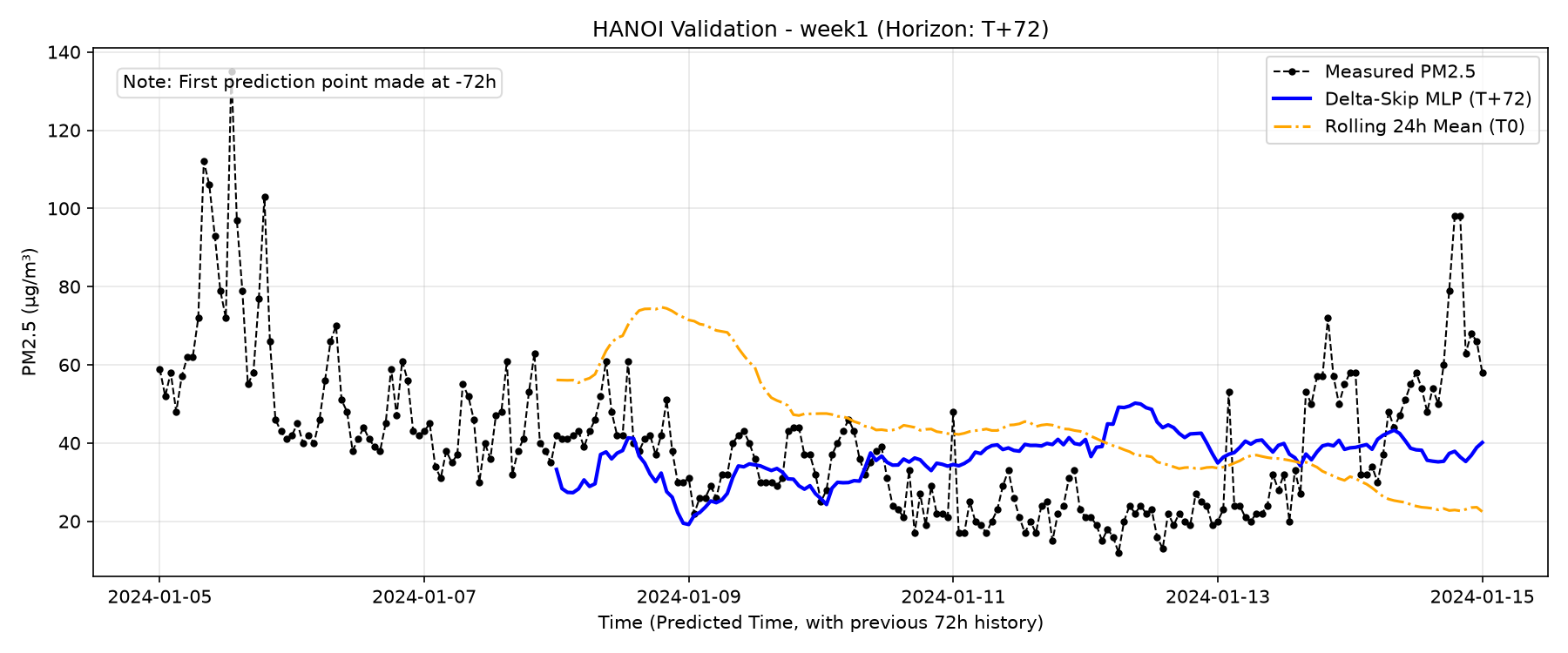
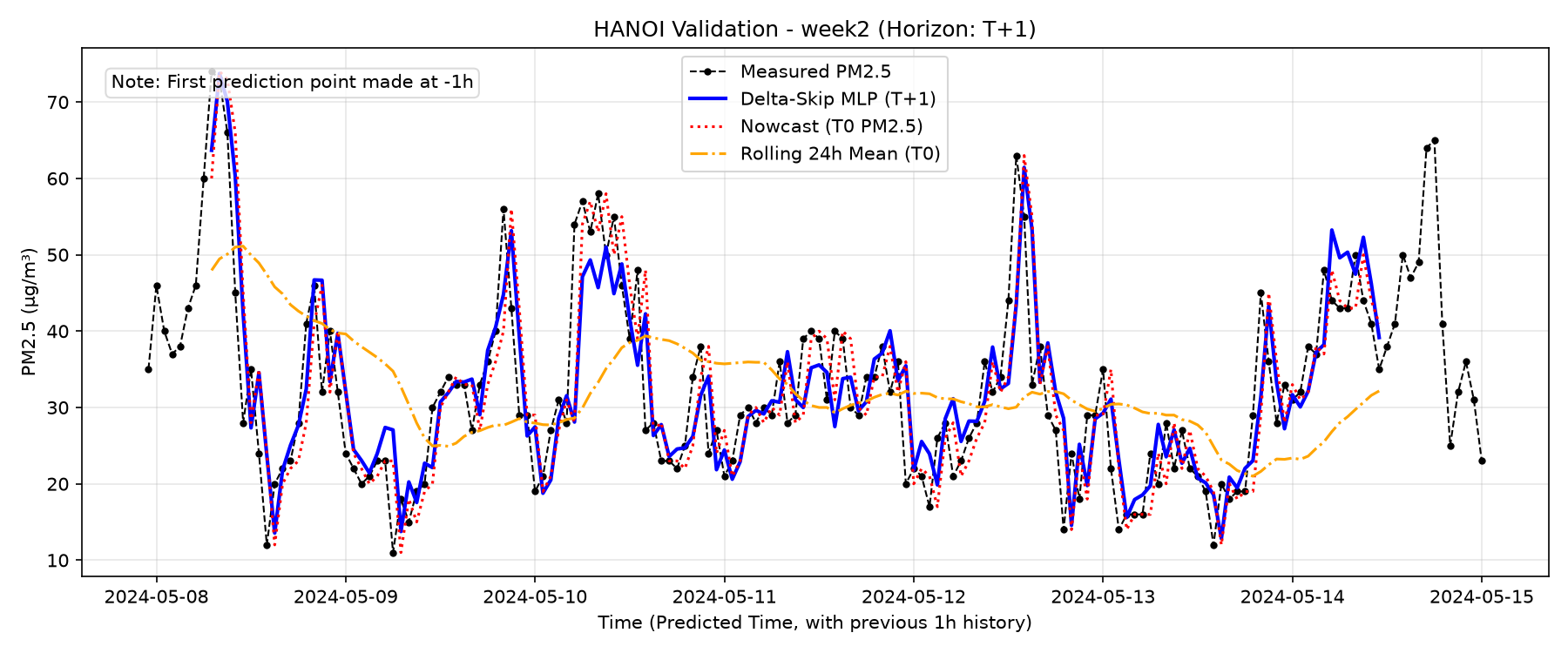
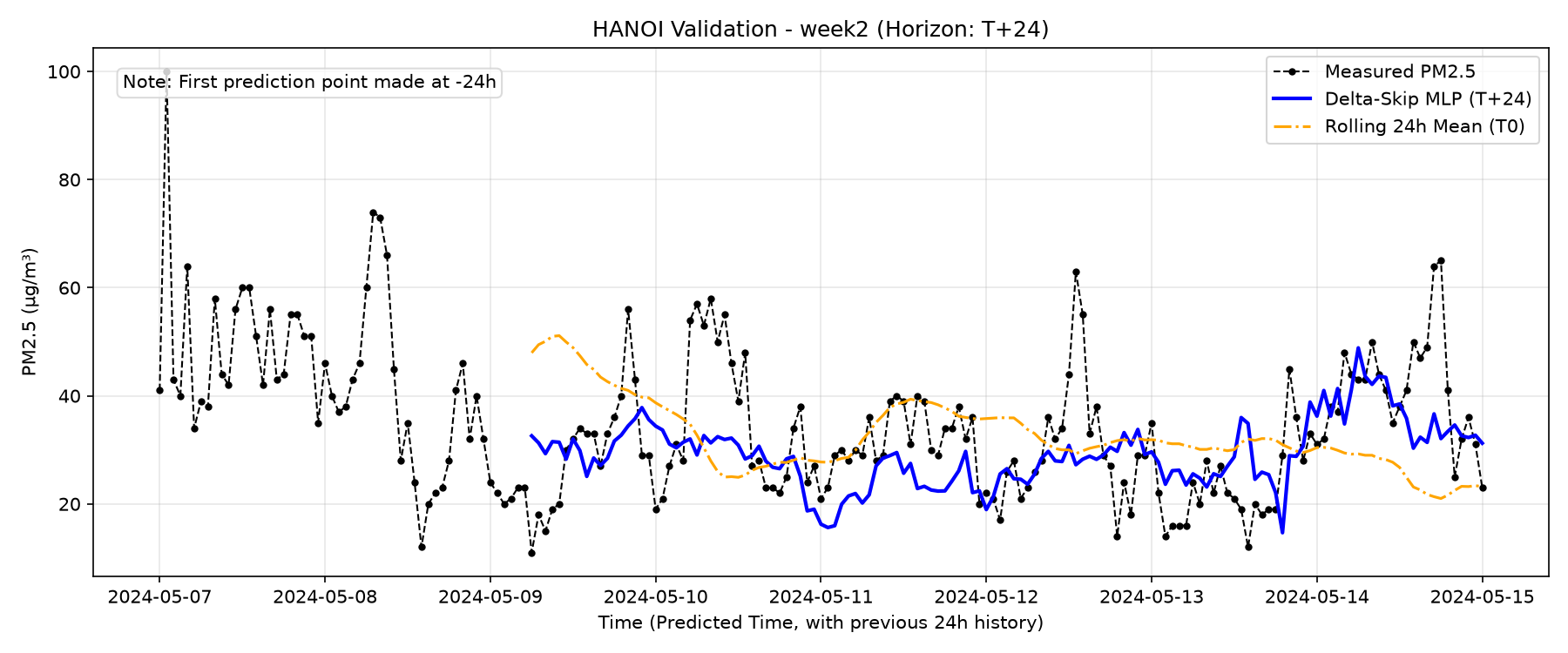
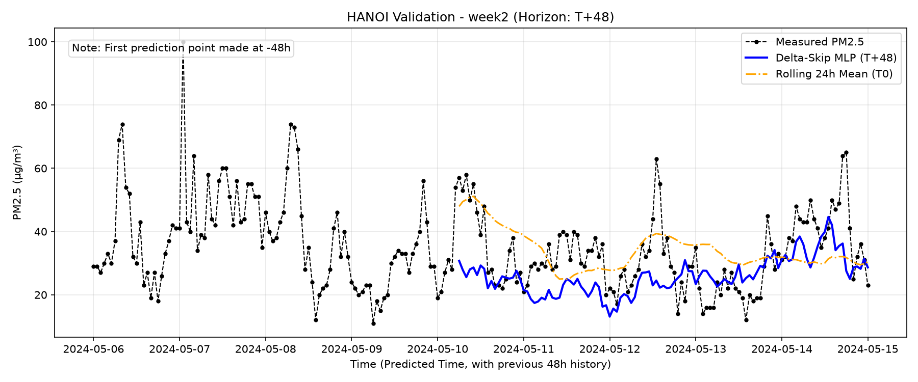
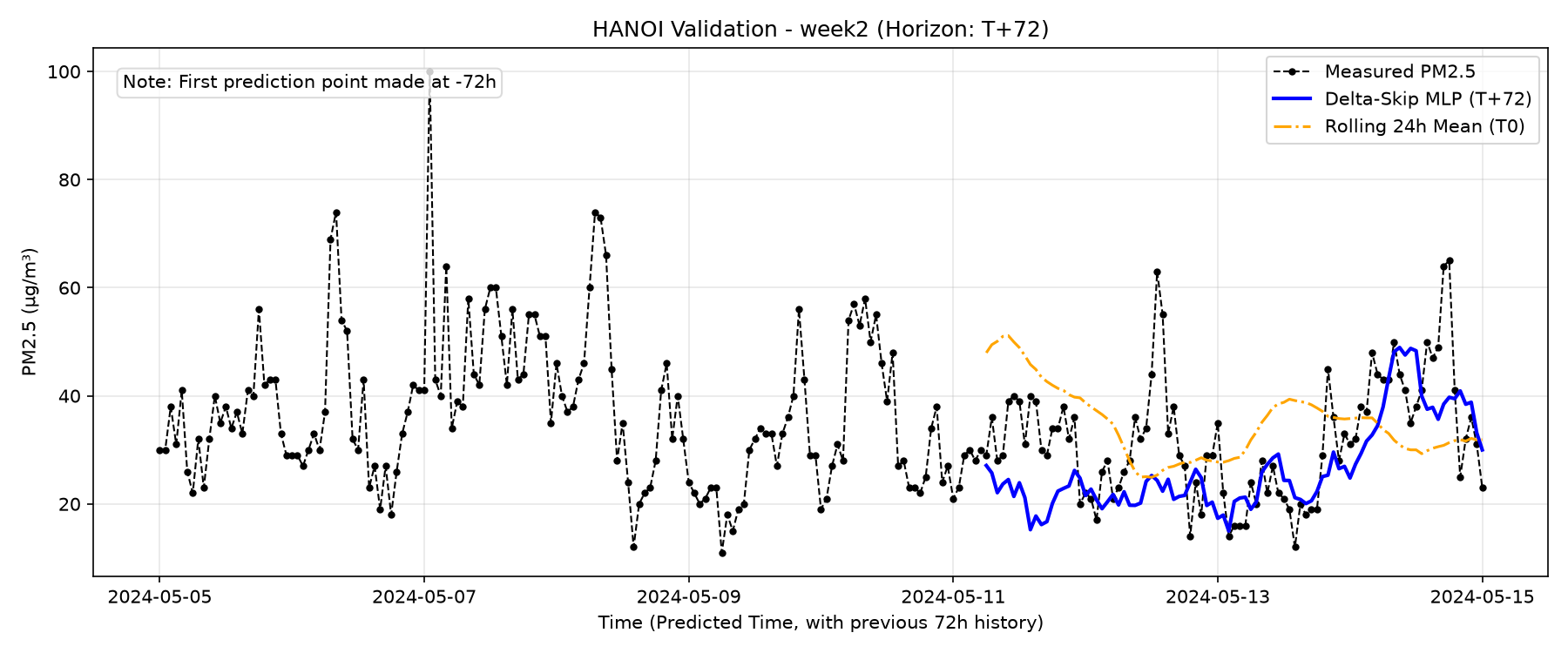
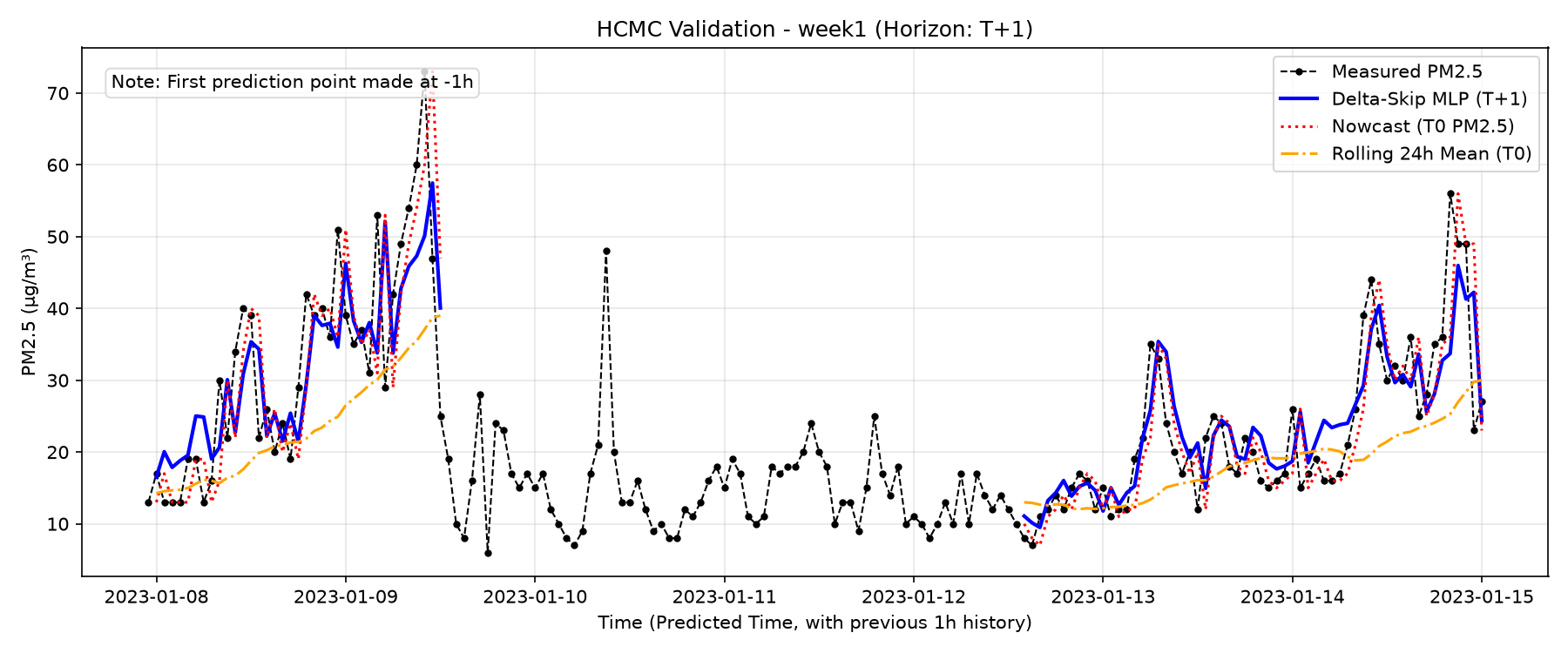
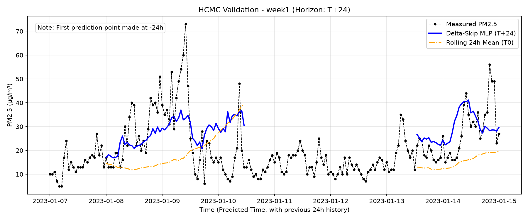
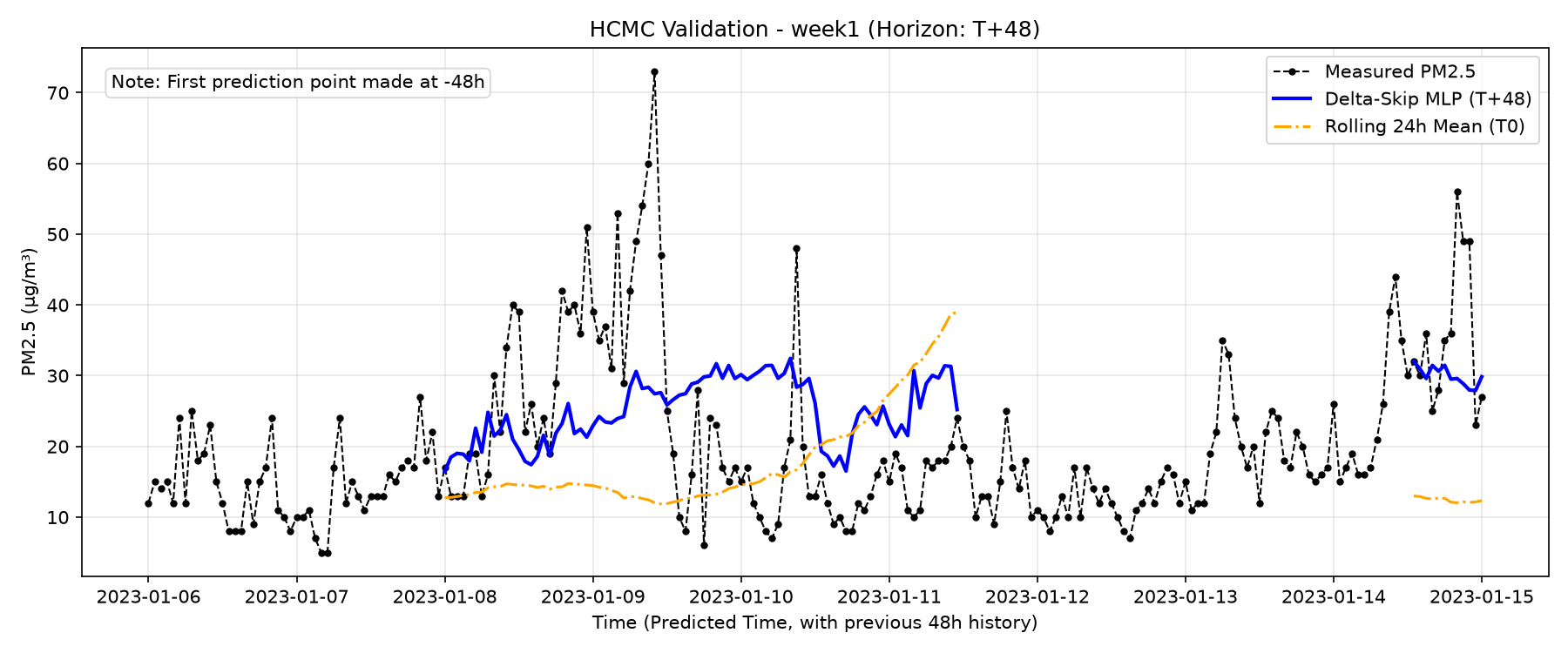
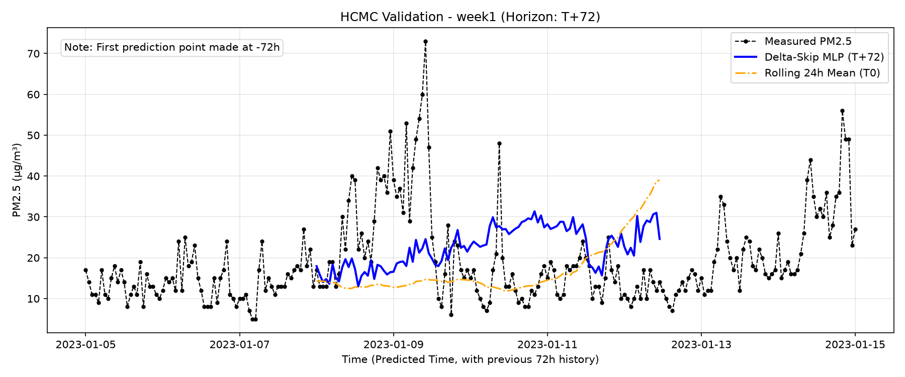
Appendix: Extended Validation Plots

The plots below visualize the operational Delta-Skip MLP forecasting 1 hour, 24 hours, and 48 hours into the future, compared against actual measurements and persistence baselines.

At T+24h and T+48h, basic rolling averages completely smooth out, missing all diurnal cycles and severe pollution spikes. The Delta-Skip MLP, driven by meteorological foresight, continues to capture the daily peaks in Hanoi and the coastal stability of HCMC days in advance.